RBM TensorFlow Implementation
Considering lack of TensorFlow implementation of RBM, I implemented one trained on MNIST data sets.
In this post, I will implement a very simple RBM, i.e., one with binary visible units and binary hidden units trained by CD-k algorithm.
I assumed readers already had enough background knowledge about RBM so I will not go into theoretical details about it. If not, please check Theano Documents and G.E.Hinton’s paper.
1. Before Start
My setting is Ubuntu 16.04 64 bit, Anaconda 4.3.1, Python 3.6, TensorFlow 1.0.0.1(CPU).
I implemented it in Jupyter Notebook.
Following a few lines of codes described packages we will use:
%matplotlib inline
import matplotlib.pyplot as plt
import numpy as np
import tensorflow as tf
import os
2. DataSet
In this implementation, I trained it on MNIST data set. So first we need to download it from here.
There should be 4 files named train-images-idx3-ubyte.gz, train-labels-idx1-ubyte.gz, t10k-images-idx3-ubyte.gz and t10k-labels-idx1-ubyte.gz each corresponding to images and labels of training set and test set.
After downloading, create a folder named mnist in your current directory and place all data files into it so as to directly run my notebook file.
2.1 Flexible Way
2.1.1 DataSet Class
In order to handle this data set easily, I create a class called DataSet to deal with them. Here are codes:
import random
import gzip, struct

class DataSet:
	batch_index = 0

	def __init__(self, data_dir, batch_size = None, one_hot = False, seed = 0):
		self.data_dir = data_dir
		X, Y = self.read()
		shape = X.shape
		X = X.reshape([shape[0], shape[1] * shape[2]])
		self.X = X.astype(np.float)/255
		self.size = self.X.shape[0]
		if batch_size == None:
			self.batch_size = self.size
		else:
			self.batch_size = batch_size
		# abandom last few samples
		self.batch_num = int(self.size / self.batch_size)
		# shuffle samples
		np.random.seed(seed)
		np.random.shuffle(self.X)
		np.random.seed(seed)
		np.random.shuffle(Y)
		self.one_hot = one_hot
		if one_hot:
			y_vec = np.zeros((len(Y), 10), dtype=np.float)
			for i, label in enumerate(Y):
				y_vec[i, Y[i]] = 1.0
			self.Y = y_vec
		else:
			self.Y = Y
The __init__ function will load the whole data set into main memory when you create a DataSet instance.
-
data_dir: a dictionary containing where and what names data files are, for instance:
train_dir = { ‘X’: ‘./mnist/train-images-idx3-ubyte.gz’, ‘Y’: ‘./mnist/train-labels-idx1-ubyte.gz’ }
- batch_size: size of mini-batch, default None means use the whole data set as a batch
- one_hot: whether labels use one-hot encoding
- seed: random seed to shuffle data
Noted that we will and will only shuffle all samples of data set once. Shuffling data will improve generalization in some sense1 , especially when we use stochastic gradient descent, which required randomly chosing a few data to compute gradients. But in practical it is hard to draw samples from a very large data set everytime we compute gradients(it need to maintain a large index array). Shuffling once will asymptotically satisfy this requirement(in expectation).
	def read(self):
		with gzip.open(self.data_dir['Y']) as flbl:
			magic, num = struct.unpack(">II", flbl.read(8))
			label = np.fromstring(flbl.read(), dtype=np.int8)
		with gzip.open(self.data_dir['X'], 'rb') as fimg:
			magic, num, rows, cols = struct.unpack(">IIII", fimg.read(16))
			image = np.fromstring(fimg.read(), dtype=np.uint8).reshape(len(label), rows, cols)
		return image,label
read function read data from files and return it. Details of this function could be safely ignored since it is irrelevant to most of things in our implementation.
	def next_batch(self):
		start = self.batch_index * self.batch_size
		end = (self.batch_index + 1) * self.batch_size
		self.batch_index = (self.batch_index + 1) % self.batch_num
		if self.one_hot:
			return self.X[start:end, :], self.Y[start:end, :]
		else:
			return self.X[start:end, :], self.Y[start:end]
The next_batch function will return data of batch which followed last batch immediately. Keep calling this function, it will automatically iterate through the whole data set and then go back to where it started.
This function will simplify codes of training main loop.
	def sample_batch(self):
		index = random.randrange(self.batch_num)
		start = index * self.batch_size
		end = (index + 1) * self.batch_size
		if self.one_hot:
			return self.X[start:end, :], self.Y[start:end, :]
		else:
			return self.X[start:end, :], self.Y[start:end]
The sample_batch function will randomly chose a batch from data set and return it.
This function is aim to simplify codes of sampling.
2.1.2 Instantiation
We can then use this class to load data:
train_dir = {
	'X': './mnist/train-images-idx3-ubyte.gz',
	'Y': './mnist/train-labels-idx1-ubyte.gz'
}

train_data = DataSet(data_dir=train_dir, batch_size=64, one_hot=True)
Noted that we use RBM to model , so actually we will not use labels, which means value of argument one_hot will not affect our training.
2.2 Simplified Way
However, despite of the above codes to handle MNIST data, we can instead reuse codes from TensorFlow’s Official Guide:
from tensorflow.examples.tutorials.mnist import input_data
mnist = input_data.read_data_sets('MNIST_data', one_hot=True)
which will significantly simplify codes and there is no need to manually download data files. But for my sake of flexibility, I decided to use my own codes.
3. Operation
Before we build our model, we need some helper functions to simplify our codes and improve readability.
def weight(shape, name='weights'):
	return tf.Variable(tf.truncated_normal(shape, stddev=0.1), name=name)

def bias(shape, name='biases'):
	return tf.Variable(tf.constant(0.1, shape=shape), name=name)
These 2 helper functions will be used to create weights and biases variables in our computation graph.
4. Model
Now we construct our RBM model, whose energy function is:
where represents the weights connecting hidden and visible units and , are the offsets of the visible and hidden layers respectively.
Noted that in our implementation, our RBM model’s units all are binary. Considering we are training on MNIST data set and after preprocessing pixels’ values are between 0 and 1, we can now interpret these values as probabilities of corresponding pixels take on values Black(1) or White(0), so that we can fit data in our model.
4.1 RBM Definition
class RBM:
	i = 0 # fliping index for computing pseudo likelihood

	def __init__(self, n_visible=784, n_hidden=500, k=30, momentum=False):
		self.n_visible = n_visible
		self.n_hidden = n_hidden
		self.k = k

		# learning rate and momentum
		self.lr = tf.placeholder(tf.float32)
		if momentum:
			self.momentum = tf.placeholder(tf.float32)
		else:
			self.momentum = 0.0

		# weights and biases
		self.w = weight([n_visible, n_hidden], 'w')
		self.hb = bias([n_hidden], 'hb')
		self.vb = bias([n_visible], 'vb')

		# velocities of momentum method
		self.w_v = tf.Variable(tf.zeros([n_visible, n_hidden]), dtype=tf.float32)
		self.hb_v = tf.Variable(tf.zeros([n_hidden]), dtype=tf.float32)
		self.vb_v = tf.Variable(tf.zeros([n_visible]), dtype=tf.float32)
__init__ function take on 4 arguments:
- n_visible: number of visible units, default is 784, which is 28*28
- n_hidden: number of hidden units, default is 500
- k: k of CD-k algorithm, default is 30
- momentum: whether to use momentum, default is False
For those who already have some experience of using TensorFlow, it should be easy to be understanded. But there are a few points I want to mentioned:
- For learning rate lr and momentum momentum, I make placeholders for them rather than fix them as constants
- k is no need to be as large as 30, sometimes 15 would be enough
- n_hidden is also no need to be as large as 500, sometimes 100 would give a model with reasonable quality but consume less training time
The reason why I use learning rate and momentum as placeholders instead of constants is that in some literatures they will dynamically decrease learning rate during training. So using placehoder will give advantages for this circumstance.
4.2 Conditional Distribution
	def propup(self, visible):
		pre_sigmoid_activation = tf.matmul(visible, self.w) + self.hb
		return tf.nn.sigmoid(pre_sigmoid_activation)

	def propdown(self, hidden):
		pre_sigmoid_activation = tf.matmul(hidden, tf.transpose(self.w)) + self.vb
		return tf.nn.sigmoid(pre_sigmoid_activation)
The propup and propdown function compute 2 and respectively.
prop is abbreviation of propagation.
When computing , we need to clamp . Viewing from picture below, this computation seems need to propagate “up”, so cames the up in function’s name(Image adopted from Theano Documents).
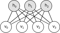
The same reason also apply to origin of down in function’s name.
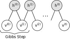
4.3 Gibbs Sampling Steps
	def sample_h_given_v(self, v_sample):
		h_props = self.propup(v_sample)
		h_sample = tf.nn.relu(tf.sign(h_props - tf.random_uniform(tf.shape(h_props))))
		return h_sample

	def sample_v_given_h(self, h_sample):
		v_props = self.propdown(h_sample)
		v_sample = tf.nn.relu(tf.sign(v_props - tf.random_uniform(tf.shape(v_props))))
		return v_sample
Above 2 functions draw samples from and respectively. They will be used in CD-k algorithm.
4.4 Learning Step
4.4.1 CD-k Algorithm
	def CD_k(self, visibles):
		# k steps gibbs sampling
		v_samples = visibles
		h_samples = self.sample_h_given_v(v_samples)
		for i in range(self.k):
			v_samples = self.sample_v_given_h(h_samples)
			h_samples = self.sample_h_given_v(v_samples)

		h0_props = self.propup(visibles)
		w_positive_grad = tf.matmul(tf.transpose(visibles), h0_props)
		w_negative_grad = tf.matmul(tf.transpose(v_samples), h_samples)
		w_grad = (w_positive_grad - w_negative_grad) / tf.to_float(tf.shape(visibles)[0])
		hb_grad = tf.reduce_mean(h0_props - h_samples, 0)
		vb_grad = tf.reduce_mean(visibles - v_samples, 0)
		return w_grad, hb_grad, vb_grad
CD_k function is the implementation of CD-k algorithm which compute gradient w.r.t weights and biases.
The k-step gibbs sampling within this algorithm could be illustracted as picture below(Image adopted from Theano Documents):
The formula to compute gradient w.r.t weights and biases is similar to the one in my previous post except the negative sign:
You can derive the particular update rule of RBM by hand according above formula.
4.4.2 Update Parameters
	def learn(self, visibles):
		w_grad, hb_grad, vb_grad = self.CD_k(visibles)
		# compute new velocities
		new_w_v = self.momentum * self.w_v + self.lr * w_grad
		new_hb_v = self.momentum * self.hb_v + self.lr * hb_grad
		new_vb_v = self.momentum * self.vb_v + self.lr * vb_grad
		# update parameters
		update_w = tf.assign(self.w, self.w + new_w_v)
		update_hb = tf.assign(self.hb, self.hb + new_hb_v)
		update_vb = tf.assign(self.vb, self.vb + new_vb_v)
		# update velocities
		update_w_v = tf.assign(self.w_v, new_w_v)
		update_hb_v = tf.assign(self.hb_v, new_hb_v)
		update_vb_v = tf.assign(self.vb_v, new_vb_v)

		return [update_w, update_hb, update_vb, update_w_v, update_hb_v, update_vb_v]
learn function will call CD_k to obtain gradients, then update weights and biases based on these gradients and momentum. Operations it returned should be run by TensorFlow’s Session with appropriate feed dictionary.
Velocity update rule:
Parameter update rule with momentum:
Parameter update rule without momentum:
These 2 update rules for parameter become equivalent when setting to 0, which is also the trick I employed in my implementation.
Postive sign inside update rule came from fact that we are doing gradient ascent.
4.5 Tracking
4.5.1 Images Sampler
	def sampler(self, visibles, steps=5000):
		v_samples = visibles
		for step in range(steps):
			v_samples = self.sample_v_given_h(self.sample_h_given_v(v_samples))
		return v_samples
sampler function will be used to draw samples from our RBM model in order to check our model’s quality visually.
Argument steps is the number of steps for markov chain to burn in, default is 500, but actually in most cases after 3000 steps the chain will mix very well.
4.5.2 Pseudo Likelihood
	def free_energy(self, visibles):
		first_term = tf.matmul(visibles, tf.reshape(self.vb, [tf.shape(self.vb)[0], 1]))
		second_term = tf.reduce_sum(tf.log(1 + tf.exp(self.hb + tf.matmul(visibles, self.w))), axis=1)
		return - first_term - second_term
free_energy function compute free energy of our model w.r.t corresponding inputs, i.e., visibles units configuration.
It followed this formula:
It will be used to compute pseudo likelihood.
	def pseudo_likelihood(self, visibles):
		x = tf.round(visibles)
		x_fe = self.free_energy(x)
		split0, split1, split2 = tf.split(x, [self.i, 1, tf.shape(x)[1] - self.i - 1], 1)
		xi = tf.concat([split0, 1 - split1, split2], 1)
		self.i = (self.i + 1) % self.n_visible
		xi_fe = self.free_energy(xi)
		return tf.reduce_mean(self.n_visible * tf.log(tf.nn.sigmoid(xi_fe - x_fe)), axis=0)
pseudo_likelihood will compute pseudo log-likelihood w.r.t corresponding inputs(This function name is inappropriate, it should be pseudo_log_likelihood).
In order to track the training process, we need to know whether our training progress during training. Since we are maximizing , by viewing how change it will tell us whether training is in the right track.
However, computing such marginal distribution require summing over all possible hidden units configurations in which there are exponential number of members. So we use pseudo log-likelihood instead of real log-likelihood.
For RBM, the corresponding pseudo log-likelihood formula is:
where is the same visible units configuration as except the i-th unit is flipped(0->1, 1->0).
For derivation details, please refer to Theano Documents.
5. Main Loop
5.1 Images Saver
Before we start our main loop of training, we need a function to save images sampled during training:
import scipy.misc

def save_images(images, size, path):
	img = (images + 1.0) / 2.0
	h, w = img.shape[1], img.shape[2]

	merge_img = np.zeros((h * size[0], w * size[1]))

	for idx, image in enumerate(images):
		i = idx % size[1]
		j = idx // size[1]
		merge_img[j*h:j*h+h, i*w:i*w+w] = image

	return scipy.misc.imsave(path, merge_img)
The best size number is
int(max(sqrt(image.shape[0]),sqrt(image.shape[1]))) + 1
Here are 2 examples:
- The batch_size is 64, then the size is recommended [8, 8]
- The batch_size is 32, then the size is recommended [6, 6]
5.2 Training Function
Now we set up our training function:
def train(train_data, epoches):
	# directories to save samples and logs
	logs_dir = './logs'
	samples_dir = './samples'

	# markov chain start state
	noise_x, _ = train_data.sample_batch()

	# computation graph definition
	x = tf.placeholder(tf.float32, shape=[None, 784])
	rbm = RBM()
	step = rbm.learn(x)
	sampler = rbm.sampler(x)
	pl = rbm.pseudo_likelihood(x)

	saver = tf.train.Saver()
After construction of computation graph, we start training main loop.
In this loop, we draw samples for every 500 batches, saved model and computed pseudo log-likelihood for every epoch. When training finished, we will draw samples from trained model for evaluation.
	# main loop
	with tf.Session() as sess:
		mean_cost = []
		epoch = 1
		init = tf.global_variables_initializer()
		sess.run(init)
		for i in range(epoches * train_data.batch_num):
			# draw samples
			if i % 500 == 0:
				samples = sess.run(sampler, feed_dict = {x: noise_x})
				samples = samples.reshape([train_data.batch_size, 28, 28])
				save_images(samples, [8, 8], os.path.join(samples_dir, 'iteration_%d.png' % i))
				print('Saved samples.')
			batch_x, _ = train_data.next_batch()
			sess.run(step, feed_dict = {x: batch_x, rbm.lr: 0.1})
			cost = sess.run(pl, feed_dict = {x: batch_x})
			mean_cost.append(cost)
			# save model
			if i is not 0 and train_data.batch_index is 0:
				checkpoint_path = os.path.join(logs_dir, 'model.ckpt')
				saver.save(sess, checkpoint_path, global_step = epoch + 1)
				print('Saved Model.')
			# print pseudo likelihood
			if i is not 0 and train_data.batch_index is 0:
				print('Epoch %d Cost %g' % (epoch, np.mean(mean_cost)))
				mean_cost = []
				epoch += 1

		# draw samples when training finished
		print('Test')
		samples = sess.run(sampler, feed_dict = {x: noise_x})
		samples = samples.reshape([train_data.batch_size, 28, 28])
		save_images(samples, [8, 8], os.path.join(samples_dir, 'test.png'))
		print('Saved samples.')
This training function should be easy to understand. But still there are a few points I need to mention:
- We use the same markov chain start state noise_x during training, and it is sampled from data set
- Learning Rate rbm.lr need to be specified at each call of sess.run as well as batch data
- Before you call this function, you need to create 2 folder named logs and samples in your current directory
For the first point, using the same start state during training won’t affect the final result since as the chain mixed, samples we draw will become irrelevant to where the chain started. As for this state is sampled from data set, it actually could be set to any value between 0 and 1. But using true data as start state, it seems that it will reduce mixing time(personally think).
For the second point, since we need to feed in learning rate, we can decrease learning rate during training(but I didn’t do it here, because constant 0.1 learning rate will give a fairly good model) which official implementations of various optimizers does not permit.
For the third point, if you didn’t do so, you will get a not found exception. This problem can be very easily handled by try-catch block/os.path.exists and os.makedirs method. But for the sake of code simplicity, I didn’t add it here.
6. Result
After doing so much works, we can finally train our model with following one line of code:
train(train_data, 50)
It take me roughly 2 more hours to finish training. In fact, we don’t need 50 epoches, 30~40 would be sufficient, as we will see soon.
6.1 During Training
6.1.1 Samples
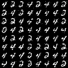
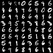
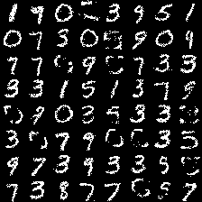
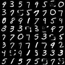
In pictures below(samples from iteration 0, 1000 and 30000), we can see that how our model learn better and better:
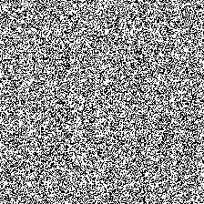
At iteration 0, our model haven’t learn anything yet, so it can only produce purely random noise.
At iteration 1000, our model already learn the concepts of background and strokes or basic form of digits, but still very blur.
At iteration 30000, our model is kind of modeling quite well. Most of its samples are highly recognizable digits.
6.1.2 Learning Curve
Picture below show how pseudo log-likelihood change during learning. As we can see, pseudo log-likelihood keep rising as we expected, since we are maximizing log-likelihood.
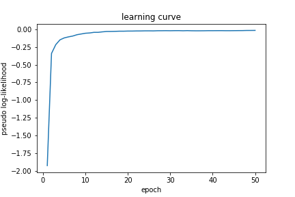
Noted that at 30~40 epoch, learning become stable, so 30~40 epoches would be enough to train our model.
To further push up this bound, one can try to use model with larger capacity, better tuned hyper-parameters or more advanced techniques like momentum to overcome local optima.
The most easy thing you can try is to reduce learning rate when approaching optima. This come from the fact that stochastic gradient descent/ascent will typically wander around local optima. Reducing learning rate more close to 0 will make it more close to local optima.
6.2 After Training
6.2.1 Samples
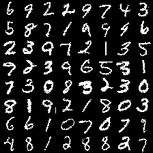
Now we draw samples from our trained model to visually check its quality:
Most of samples are highly recognizable digits. Some of them are inferior. This may be due to the lack of model capacity or mixing of markov chain is not well.
Despite of bad samples, we can see that even in samples with highly recognizable digits, they seem to have some background noise. This might probably be due to the sampling process and inherent problem within our model.
We know that for RBM its inputs is binary variables. However, our gray scale images are consisted of real values between . In this case we divide them by 255 so that their values are scaled to and can be interpreted as probability of taking corresponding varible to 0(black) or 1(white).
After finishing this preprocess procedure, we can draw samples from such distributions:
We can see that such samples are very similar to what we draw from learnt RBM. This explain that why RBM’s samples seem containing background noise: If RBM fits data distributions well, then it will output a similar distribution to draw samples, thus these samples will have similar visual effects(background noise).
If we instead rescale RBM’s output distribution and print it as a gray scale image, then we will get a better sample:
For the blur part of these images, this might be results of not mixing well of Markov Chain and low model capacity. we can improve this by allowing mixing more steps and using deeper model.
6.2.2 Filters
Picture below show weights of each hidden unit to all visible units(Image adopted from Theano Documents).
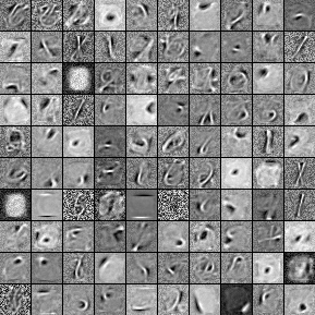
We can see that after traning, each hidden unit learn to recognize different patterns, which show like sophisticated strokes.
7. Conclusion
So far we have already implemented a very simple RBM model. However, there are many varients of RBM, such as RBM with Gussian visible units, stacked RBMs and so on. Also there are many learning algorithm for RBM, such as PCD or wake-sleep algorithm. But with knowledge of implementing this simple form of RBM, we are able to build more complex models.
The .ipynb file of codes in this post is available on my GitHub.
8. Reference
- GitHub: tensorflow-rbm
- Theano Documents: RBM
- Stackoverflow: RBM implementation
- A Practical Guide to Training RBM, G.E.Hinton
- EBM Notes, Yanyang Lee
9. Appendix
- Shuffling remove extra regularites introduced by the order of data. These regularities will appear in mini-batch setting, where sometimes some batches only consist of a small fraction of possible categories, which will produce a biased estimate of true gradient, resulting in model learnt non-existed regularities. Go Back
- Because of some unknown mistakes in jekyll, we can’t present P(h|v) but P(h||v) via MathJax sometimes. Go Back