This note is meant to remind readers some important properties or conclusions about EBMs, i.e., energy-based models.

To read through this note, you might need some background knowledge about EBMs, RBMs and MRFs. This note is not for newbie but for those only knew some basic concepts of these models and want to know more mathematics underlying them or those had troubles in understanding mathematics of these models.

1. Joint Distribution

For random variables within EBMs, they can usually be divided into 2 sets. Some random variables’ values can be observed, and we denoted them as $v$, i.e., visible. Others can not be observed, and we denoted them as $h$, i.e., hidden.

Here, $h$ and $v$ are vectors whose elements are correspond to activities of certain units.

We denoted Energy of a specific configuration $(h,v)$ as $E(h,v)$. $E$ function can take on any real value.

For a specific configuration $(h,v)$, its corresponding probability is:

$$P(h,v)=\frac{e^{-E(h,v)}}{Z}$$

where $Z$ is normalization constant, $Z=\sum_{h,v} e^{-E(h,v)}$.

Using $e^{-E}$ ensure the unnormalized distribution is always postive, and free the energy function to take on any real value.

2. Marginal Distribution

Some times we want to know $P(v)$:

$$P(v)=\sum_h P(h,v)=\frac{\sum_h e^{-E(h,v)}}{Z}$$

3. Maximun log-Likelihood

For the learning problem of EBMs, we always want to use optimization algorithms, like gradient descent, to:

$$argmin_\theta -log\ P(v;\theta)$$

or more formally,

$$argmin_\theta -\sum_v log\ P(v;\theta)$$

for all $v$ from training set.

Thus we need to compute $\frac{\partial -log\ P(v;\theta)}{\partial \theta}$ in order to perform updates.

$$\frac{\partial -log\ P(v;\theta)}{\partial \theta} = -\frac{\partial log \sum_h e^{-E(h,v)}}{\partial \theta} + \frac{\partial log\ Z}{\partial \theta}$$

Here we expand left side of equation using marginal distribution relationship between $P(v)$ and $P(h,v)$, and noted that $\theta$ is contained in energy function.

On the right side of equation, we always denote the first term $-\frac{\partial log \sum_h e^{-E(h,v)}}{\partial \theta}$ as postive phase and the second term $\frac{\partial log\ Z}{\partial \theta}$ as negative phase. Later I will describe these two terms in more details.

3.1 Postive Phase

For postive phase, we keep applying chain rule:

$$-\frac{\partial log \sum_h e^{-E(v,h)}}{\partial \theta} = - \frac{1}{\sum_h e^{-E(h,v)}} \sum_h \frac{\partial e^{-E(h,v)}}{\partial \theta} = -\frac{1}{\sum_h e^{-E(h,v)}} \sum_h e^{-E(h,v)} \frac{\partial -E(h,v)}{\partial \theta}$$

Then we move the first fraction into the summation and keep applying chain rule so that the negative sign could be cancelled out:

$$= \sum_h \frac{e^{-E(h,v)}}{\sum_h e^{-E(h,v)}} \frac{\partial E(h,v)}{\partial \theta}$$

Next we divide $Z$ from numerator and denominator of the first fraction simutaneouly so as to apply the definitions of joint distribution and marginal distribution:

$$= \sum_h \frac{\frac{e^{-E(h,v)}}{Z}}{\frac{\sum_h e^{-E(h,v)}}{Z}} \frac{\partial E(h,v)}{\partial \theta} = \sum_h \frac{P(h,v)}{P(v)}\frac{\partial E(h,v)}{\partial \theta} = \sum_h P(h|v) \frac{\partial E(h,v)}{\partial \theta}$$

We can rewrite it as a form of expectation:

$$E_{h \sim P(h|v)} \frac{\partial E(h,v)}{\partial \theta}$$

This is the final form of postive phase.

Warning: Noted that we abuse notation $h$ since it no longer represent a random variable instead a specific value of this random variable. Replacing it with other symbols will be more appropriate but less straightforward.

3.2 Negative Phase

For negative Phase, we also keep applying chain rule:

$$\frac{\partial log\ Z}{\partial \theta} = \frac{1}{Z} \frac{\partial Z}{\partial \theta}$$

Subsitute $Z$ with its definition $Z=\sum_{h,v} e^{-E(h,v)}$ and apply chain rule again:

$$= \frac{1}{Z} \sum_{h',v'} \frac{\partial e^{-E(h',v')}}{\partial \theta} = \frac{1}{Z} \sum_{h',v'} e^{-E(h',v')} \frac{\partial -E(h',v')}{\partial \theta} = -\frac{1}{Z} \sum_{h',v'} e^{-E(h',v')} \frac{\partial E(h',v')}{\partial \theta}$$

Move the first fraction into summation so that we can use definition of joint distribution:

$$= -\sum_{h',v'} \frac{e^{-E(h',v')}}{Z} \frac{\partial E(h',v')}{\partial \theta} = -\sum_{h',v'} P(h',v') \frac{\partial E(h',v')}{\partial \theta}$$

We can also rewrite it as a form of expectation:

$$-E_{h',v' \sim P(h,v)} \frac{\partial E(h',v')}{\partial \theta}$$

3.3 Learning Rule

At last, we obtained:

$$\frac{\partial -log\ P(v;\theta)}{\partial \theta} = E_{h \sim P(h|v)} \frac{\partial E(h,v)}{\partial \theta} - E_{h',v' \sim P(h,v)} \frac{\partial E(h',v')}{\partial \theta}$$

Noted that name of these two terms did not come from their sign, but come from the fact that for postive phase, $h \sim P(h\|v)$ 1 where $P(h\|v)$ is defined by $\theta$ and $h$ is free but $v$ is given by training set, and for negative phase, $h',v' \sim P(h,v)$ where $P(h,v)$ is defined by $\theta$ but $v'$ and $h'$ are free.

4. Details in RBMs

Restricted Boltzmann Machine, known as RBMs, is a particular variant of EBMs.

RBMs shared all properties that EBMs have, but there is a few details that we should look at.

4.1 Energy Function

For RBMs, its energy function take on a specific form:

$$E(h,v) = -v^TWh-b^Tv-c^Th$$

where $W$ is weight matrix, $W_{ij}$ means weight on connection from visible unit $i$ to hidden unit $j$.

4.2 Posterior Distribution

According to EBM learning rule, we need to know $P(h\|v)$. In RBMs, it has a easy-to-compute form:

$$P(h|v) = \frac{P(h,v)}{P(v)}$$ $$= \frac{\frac{e^{-E(h,v)}}{Z}}{\frac{\sum_h e^{-E(h,v)}}{Z}}$$ $$= \frac{e^{-E(h,v)}}{\sum_h e^{-E(h,v)}}$$ $$= \frac{e^{b^Tv+c^Th+v^TWh}}{\sum_h e^{b^Tv+c^Th+v^TWh}}$$

We can cancel all terms that didn’t contain $h$ using property of exp:

$$= \frac{e^{b^Tv} e^{c^Th+v^TWh}}{\sum_h e^{b^Tv}e^{c^Th+v^TWh}}$$ $$= \frac{e^{b^Tv} e^{c^Th+v^TWh}}{e^{b^Tv} \sum_h e^{c^Th+v^TWh}}$$ $$= \frac{e^{c^Th+v^TWh}}{\sum_h e^{c^Th+v^TWh}}$$

Now we can treat the denominator as normalization constant:

$$= \frac{e^{c^Th+v^TWh}}{Z'}$$ $$= \frac{exp\big\{\sum_{j=1}^{n_h} c_jh_j + \sum_{j=1}^{n_h} v^TW_{:,j}h_j \big\}}{Z'}$$ $$= \frac{\prod_{j=1}^{n_h} exp\big\{c_jh_j + v^TW_{:,j}h_j\big\}}{Z'}$$

where $n_h$ is the number of hidden units.

This form of $P(h\|v)$ tells us its factorial nature because of the product of unnormalized distribution over the individual elements $h_j$.

If all random variables in RBM are binary variables, we can derive that:

$$P(h_j=1|v) = \frac{P'(h_j=1|v)}{P'(h_j=0|v)+P'(h_j=1|v)}$$ $$= \frac{exp\big\{c_j+v^TW_{:,j}\big\}}{exp\big\{0\big\}+exp\big\{c_j+v^TW_{:,j}\big\}}$$ $$= sigmoid(c_j+v^TW_{:,j})$$

where $P'$ denotes the unnormalized distribution.

Because of the factorial nature of $P(h\|v)$, we can write it into this form:

$$P(h|v)=\prod_{j=1}^{n_h} sigmoid\big((2h-1) \cdot (c+W^Tv)\big)_j$$

Similarly,

$$P(v|h)=\prod_{i=1}^{n_v} sigmoid\big((2v-1) \cdot (b+Wh)\big)_i$$

where $\cdot$ denotes a element-wise product operation.

4.3 Relation to MRF

RBM is actually a log-linear Markov Random Field, i.e., MRF. I won’t present definition of MRF here but only a picture to describe their relationship.

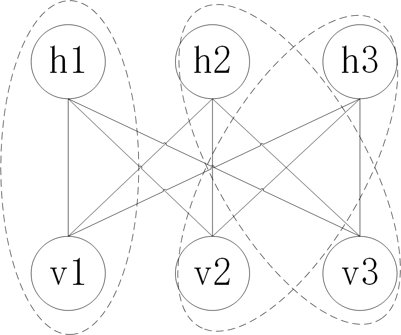
For each clique functions, they have the same form:

$$\phi(v_i,h_j)=e^{W_{ij}v_ih_j+b_iv_i+c_jh_j}$$

5. Reference

1. Deep Learning, Goodfellow et al., MIT Press.
2. Neural Networks for Machine Learning, Hinton et al., Coursera.
3. Restricted Boltzmann machine, Wikipedia.
4. Restricted Boltzmann Machines (RBM), DeepLearning 0.1 documentation.
5. Deep Learning Short Course: 4-Connection, Yanyang Lee, GitHub.

6. Appendix

1. Because of some unknown mistakes in jekyll, we can’t present P(h|v) but P(h||v) via MathJax sometimes. Go Back